Uke 00: Vektorkalkulus
Læringsmål
Denne uken skal vi lære grunnleggende elementer i vektor-kalkulus, slik at du er i stand til å kunne regne ut gradienter, divergens og kurl, løse volum, overflate og linjeintergraler, og bruke divergensteoremet og Stokes teorem i teoretiske utledninger.Diskusjonsoppgaver for gruppene
Exercise 1.1: Manhattan-norm
We have introduced the norm of a vector \( (a_x,a_y,a_z) \) as \( \sqrt{a_x^2 + a_y^2 + a_z^2} \). We call this the Euclidian norm or the \( L2 \) norm. In general we can introduce the \( Lk \) norm for an integer \( k \) as $$ \begin{equation} |\vec{a}|_k = \left( |a_x|^k + |a_y|^k + |a_z|^k\right)^{1/k} \tag{1.1} \end{equation} $$ Why do you think that the \( L1 \) norm is often called the Manhattan norm? How would you interpret the \( L0 \) norm? And what does the \( L\infty \)-norm correspond to?
Gruppeoppgaver
Exercise 1.2: Vector sums
Fig. 1a shows two vectors \( \vec{a} \) and \( \vec{b} \) each of length \( 1 \text{m} \).
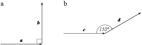 |
Figure 1: Two vectors. |
a) Draw the vector \( \vec{A} = \vec{a} + \vec{b} \).
b) Find \( \vec{a}\cdot \vec{b} \).
0
We notice that since they are orthogonal, the dot product is zero.
c) Find the length of \( \vec{a} + \vec{b} \).
\( \sqrt{2} \, \text{m} \)
We find the length by applying the definition $$ \begin{equation} |\vec{a}+ \vec{b}| = \sqrt{(\vec{a}+ \vec{b})\cdot (\vec{a}+ \vec{b})} = \sqrt{|\vec{a}|^2 + 2 \vec{a}\cdot \vec{b} + |\vec{b}|^2}=\sqrt{1 + 1} \, \text{m} = \sqrt{2} \, \text{m} \; . \tag{1.2} \end{equation} $$
Fig. 1b shows two vectors \( \vec{c} \) and \( \vec{d} \) each of length \( 1 \text{m} \).
d) Draw the vector \( \vec{c} + \vec{d} \).
e) Find \( \vec{c} \cdot \vec{d} \).
\( \sqrt{3}/2 \, \text{m}^2 \)
Notice that the correct angle to use is \( 30^{\circ} \) and not \( 150^{\circ} \). However, does this really matter? We find this by applying the definition: $$ \begin{equation} \vec{c} \cdot \vec{d} = |\vec{c}||\vec{d}| \cos \theta = 1 \text{m} \, 1 \text{m} \, \cos 30^{\circ} = 1 \text{m}^2 \frac{1}{2}\sqrt{3} = \frac{\sqrt{3}}{2}\, \text{m}^2\; . \tag{1.3} \end{equation} $$
f) Find the length of \( \vec{c} + \vec{d} \)
\( \sqrt{2+\sqrt{3}/2}\, \text{m} \)
We find the length by applying the definition $$ \begin{equation} |\vec{c}+ \vec{d}| = \sqrt{(\vec{c}+ \vec{d})\cdot (\vec{c}+ \vec{d})} = \sqrt{|\vec{c}|^2 + 2 \vec{c}\cdot \vec{d} + |\vec{d}|^2}=\sqrt{1 + 1 + \frac{\sqrt{3}}{2} \, \text{m}^2} = \sqrt{2+\sqrt{3}/2}\, \text{m}\; . \tag{1.4} \end{equation} $$
Assume that the unit vectors for a coordinate system are \( \x = \vec{a}/|\vec{a}| \) and \( \y = \vec{b}/|\vec{b}| \) and that \( \vec{c} = \vec{a} \).
g) What is \( \vec{c} \cdot \x \), \( \vec{c} \cdot \y \), \( \vec{d} \cdot \x \), and \( \vec{d} \cdot \y \)?
\( \vec{c} \cdot \x = 1 \text{m} \), \( \vec{c} \cdot \y = 0 \), \( \vec{d} \cdot \x = \sqrt{3}/2 \, \text{m} \), \( \vec{d} \cdot \y = (1/2) \text{m} \).
We can find these using the definition of the dot product: $\vec{c} \cdot \x = \vec{c} \cdot \vec{a}/|\vec{a}| = 1 \text{m}. \( \vec{c} \cdot \y = 0 \), \( \vec{d} \cdot \x = \vec{d} \cdot \vec{c} \), \( \vec{d} \cdot \y = |\vec{d}| \, |\y| \cos \theta = 1 \cos 60^{\circ} \text{m} = (1/2) \text{m} \).
h) Write \( \vec{c} \) and \( \vec{d} \) in Cartesian coordinates, that is, on the form \( (x,y) \).
\( \vec{c} = (1,0) \, \text{m} \), \( \vec{d} = (\sqrt{3}/2,1/2) \, \text{m} \).
Exercise 1.3: Decomposition
We have two vectors in a Cartesian coordinate system: \( \vec{a} = (2,1) \) and \( \vec{b} = (2,4) \).
a) Find \( \vec{a} \cdot \vec{b} \).
8
\( \vec{a} \cdot \vec{b} = (2,1) \cdot (2,4) = 2\cdot 2 + 1 \cdot 4 = 4+4 = 8 \)
b) Explain why we can interpret \( \vec{b} \cdot \vec{a}/|\vec{a}| \) as the length of \( \vec{b} \) along \( a \).
c) We call the vector \( \vec{b}_{\vec{a}} = \vec{b} \cdot (\vec{a}/|\vec{a}|) \, (\vec{a}/|\vec{a}|) \) the projection of \( \vec{b} \) onto \( \vec{a} \). Find the projection of \( \vec{b} \) onto \( \vec{a} \).
\( (8/5)(2,1) \)
The unit vector along \( \vec{a} \) is \( \vec{a}/a = (2,1)/\sqrt{5} \). We find that \( \vec{b} \cdot \vec{a}/a = 8/\sqrt{5} \). Therefore, \( \vec{b} \cdot (\vec{a}/a) (\vec{a}/a) = 8(2,1)/5 = (8/5)(2,1) \)
d) Show that \( \vec{b} - \vec{b}_{\vec{a}} \) is orthogonal to \( \vec{a} \).
\( (\vec{b} - \vec{b}\cdot (\vec{a}/a))\cdot \vec{a} = \vec{b} \cdot \vec{a} - \vec{b} \cdot \vec{a} = 0 \)
We can show this generally. We introduce \( \vec{u} = \vec{a}/a \). $$(\vec{b} - \vec{b} \cdot \vec{u} \vec{u}) \cdot \vec{a} = \vec{a} \cdot \vec{b} - \vec{b} \cdot \vec{a}/a \vec{a}/a \cdot \vec{a} = 0 \; .$$
Exercise 1.4: Cross products of a unit vector
The Cartesian unit vectors in a three-dimensional system are \( \x = (1,0,0) \), \( \y = (0,1,0) \), \( \z = (0,0,1) \).
a) A set of vectors are called orthonormal if they all are of unit length and they are orthogonal to each other. Show that the set of unit vector \( \{ \x,\y,\z \} \) are orthonormal.
\( \x \cdot \y = (1,0,0) \cdot (0,1,0) = 0+0+0 = 0 \) and similar for the other.
We perform all dot products, noting that the vectors have no common components and therefore that all dot products are zero.
b) A sequence of three orthonormal unit vectors \( (\x,\y,\z) \) form a positively orientated coordinate system if \( \x \times \y = \z \). Show that this is true for \( (\x,\y,\z) \).
\( (1,0,0) \times (0,1,0) = (0 \, 0 - 0 \, 1 , 0\, 0-1\, 0, 1\, 1 - 0 \, 0) = (0,0,1) \)
\( (1,0,0) \times (0,1,0) = (0 \, 0 - 0 \, 1 , 0\, 0-1\, 0, 1\, 1 - 0 \, 0) = (0,0,1) \)
c) What other sequences of the unit vectors form a positively oriented coordinate system?
\( (\y,\z,\x) \), \( (\z,\x,\y) \).
Exercise 1.5: Sketching a vector field
A vector field is given as \( \vec{E}(\vec{r}) = \vec{r}/|\vec{r}|^3 \).
a) Make a sketch of the vector field in the \( xy \)-plane.
b) Write a program to plot the vector field in the \( xy \)-plane.
import numpy as np
import matplotlib.pyplot as plt
def efield(r):
    return r/np.linalg.norm(r)**3
x = np.linspace(-2,2,20)
y = np.linspace(-2,2,20)
rx,ry = np.meshgrid(x,y,indexing="ij")
Ex = rx.copy()
Ey = ry.copy()
for i in range(len(rx.flat)):
    r = np.array([rx.flat[i],ry.flat[i]])
    Ex.flat[i],Ey.flat[i] = efield(r)
plt.quiver(rx,ry,Ex,Ey)
import numpy as np
import matplotlib.pyplot as plt

def efield(r):
    return r/np.linalg.norm(r)**3

x = np.linspace(-2,2,20)
y = np.linspace(-2,2,20)
rx,ry = np.meshgrid(x,y)

Ex = rx.copy()
Ey = ry.copy()
for i in range(len(rx.flat)):
    r = np.array([rx.flat[i],ry.flat[i]])
    Ex.flat[i],Ey.flat[i] = efield(r)

plt.quiver(rx,ry,Ex,Ey)
c) A vector field is given as \( \vec{E} = \frac{3 \left( \vec{r} \cdot \vec{p}\right)\vec{r}}{r^5} - \frac{\vec{p}}{r^3} \) where \( \vec{p} = (1,0) \) and \( r = |\vec{r}| \). Write a program to visualize the vector field in the \( xy \)-plane.
p = np.array([1,0])
def efield2(r,p):
    return 3*np.dot(r,p)*r/np.linalg.norm(r)**5-p/np.linalg.norm(r)**3
x = np.linspace(-2,2,20)
y = np.linspace(-2,2,20)
rx,ry = np.meshgrid(x,y,indexing="ij")
Ex2 = rx.copy()
Ey2 = ry.copy()
for i in range(len(rx.flat)):
    r = np.array([rx.flat[i],ry.flat[i]])
    Ex2.flat[i],Ey2.flat[i] = efield2(r,p)
plt.quiver(rx,ry,Ex2,Ey2)
p = np.array([1,0])
def efield2(r,p):
    return 3*np.dot(r,p)*r/np.linalg.norm(r)**5-p/np.linalg.norm(r)**3

x = np.linspace(-2,2,20)
y = np.linspace(-2,2,20)
rx,ry = np.meshgrid(x,y,indexing="ij")

Ex2 = rx.copy()
Ey2 = ry.copy()
for i in range(len(rx.flat)):
    r = np.array([rx.flat[i],ry.flat[i]])
    Ex2.flat[i],Ey2.flat[i] = efield2(r,p)

plt.quiver(rx,ry,Ex2,Ey2)
Exercise 1.6: Fluxes
Fig. 2 shows six different surfaces \( S \) with surface normals indicated by the red vector. There is a vector field \( \vec{E} = E_0 \z \) everywhere in space. Find the flux \( \Phi \) of the vector field through the different surfaces.
Figure 2: Illustration of surfaces \( S_a \) to \( S_f \).
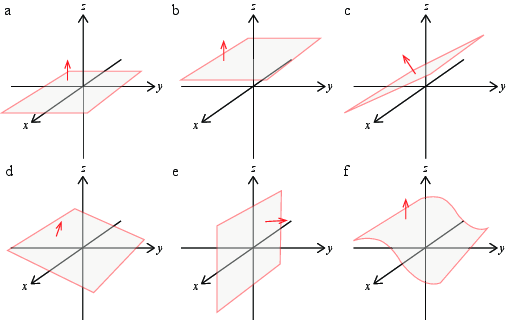
a) Surface \( S_a \) has vertices at \( (1,1,0) \), \( (-1,1,0) \), \( (1,-1,0) \) and \( (-1,-1,0) \).
\( \Phi = 4E_0 \).
b) Surface \( S_b \) has vertices at \( (1,1,1) \), \( (-1,1,1) \), \( (1,-1,1) \) and \( (-1,-1,1) \).
\( \Phi = 4 E_0 \)
c) Surface \( S_c \) has vertices at \( (1,1,1) \), \( (-1,1,1) \), \( (1,-1,0) \) and \( (-1,-1,0) \).
\( \Phi = 4 E_0 \)
Notice thas it is only the cross-sectional area, that is the area in the plane normal to the normal vector, that counts when the field is uniform. This is the same as above.
d) Surface \( S_d \) has vertices at \( (1,1,0) \), \( (-1,1,0) \), \( (1,-1,1) \) and \( (-1,-1,1) \).
\( \Phi = 4 E_0 \)
Notice thas it is only the cross-sectional area, that is the area in the plane normal to the normal vector, that counts when the field is uniform. This is the same as above.
e) Surface \( S_e \) has vertices at \( (1,0,1) \), \( (-1,0,1) \), \( (1,0,-1) \) and \( (-1,0,-1) \).
\( \Phi = 0 \)
The surface \( \vec{S} = S \nhat \), where \( \nhat = \y \). Therefore \( \vec{E} \cdot \vec{S} = 0 \).
f) Surface \( S_f \) has vertices at \( (1,1,0) \), \( (-1,1,0) \), \( (1,-1,1) \) and \( (-1,-1,1) \).
\( \Phi = 4 E_0 \)
Notice thas it is only the cross-sectional area, that is the area in the plane normal to the normal vector, that counts when the field is uniform. This is the same as above, even if the surface has a complicated shape.
Exercise 1.7: Gradients
Find the gradients of the folling scalar fields
a) \( V(x,y) = V_0 x \)
\( \nabla V = V_0 \x \)
b) \( V(x,y) = V_0 \sin x \)
\( \nabla V = V_0 \cos \x \, \x \)
c) \( V(x,y,z) = V_0 (x+y-z) \)
\( \nabla V = V_0(1,1,-1) \)
d) \( V(r) = r^2 = (x^2 + y^2 + z^2) \)
\( \nabla V = (2x,2y,2z) \)
e) \( V(r) = r = (x^2 + y^2 + z^2)^{1/2} \)
\( \nabla V = \vec{r}/|\vec{r}| \)
We see that $$ \begin{equation*} \frac{\partial V}{\partial x} = 2 x \left( x^2 + y^2 + z^2 \right)^{-1/2} \, \left( \frac{1}{2} \right) = \frac{x}{r} \; , \end{equation*} $$ with similar results for the \( y \) and \( z \) coordinates, giving $$ \begin{equation} \nabla V = \left( \frac{\partial V}{\partial x}, \frac{\partial V}{\partial y}, \frac{\partial V}{\partial z}\right) = \left(\frac{x}{r}, \frac{y}{r} ,\frac{z}{r}\right) = \frac{\vec{r}}{r} = \rhat \; . \tag{1.6} \end{equation} $$
f) \( V(r) = V_0/r \)
\( \nabla V = -V_0\frac{\vec{r}}{r^3} \)
We start by finding the \( x \)-component: $$ \begin{equation*} \frac{\partial V}{\partial x} = V_0 \frac{\partial}{\partial x} \left( x^2 + y^2 + z^2 \right)^{-1/2} = 2 x \left( x^2 + y^2 + z^2 \right)^{-3/2} \, \left( -\frac{1}{2} \right) = -\frac{x}{r^3} \; , \end{equation*} $$ with similar results for the \( y \) and \( z \) coordinates, giving $$ \begin{equation*} \nabla V = \left( \frac{\partial V}{\partial x}, \frac{\partial V}{\partial y}, \frac{\partial V}{\partial z}\right) = V_0\left(-\frac{x}{r^3}, -\frac{y}{r^3} ,-\frac{z}{r^3}\right) = -V_0\frac{\vec{r}}{r^3} = -\frac{V_0}{r^2}\rhat \; . \end{equation*} $$
Exercise 1.8: Divergence and curl
Find the divergence and curl of the following vector fields
a) \( \vec{E} = (1,0,0) \)
\( \nabla \cdot \vec{E} = 0 \), \( \nabla \times \vec{E} = \vec{0} \)
b) \( \vec{E} = \vec{r} = (x,y,z) \)
\( \nabla \cdot \vec{E} = 3 \), \( \nabla \times \vec{E} = \vec{0} \)
c) \( \vec{E} = (x,y,-2z) \)
\( \nabla \cdot \vec{E} = 0 \), \( \nabla \times \vec{E} = \vec{0} \)
d) \( \vec{E} = (-y,x,0) \)
\( \nabla \cdot \vec{E} = 0 \), \( \nabla \times \vec{E} = (0,0,2) \)
e) \( \vec{E} = \nabla V_0e^{-y}\sin x \)
\( \nabla \cdot \vec{E} = 0 \), \( \nabla \times \vec{E} = \vec{0} \)
f) \( \vec{E} = \vec{r}/r^3 \)
\( \nabla \cdot \vec{E} = 0 \), \( \nabla \times \vec{E} = \vec{0} \)
To find the divergence, we first calculuate $$ \begin{equation*} \frac{\partial E_x}{\partial x} = \frac{\partial}{\partial x} \left( xr^{-3}\right) = r^{-3} + xr^{-4}(-3)\frac{\partial r}{\partial x} = r^{-3}- 3\frac{x^2}{r^5} \; , \end{equation*} $$ where we have used that \( \partial r/\partial x = x/r \). We sum together each component, getting: $$ \begin{equation} \nabla \cdot \frac{\vec{r}}{r^3} = r^{-3} - 3\frac{x^2}{r^5} + r^{-3} - 3\frac{y^2}{r^5} + r^{-3} - 3\frac{z^2}{r^5} = 3 r^{-3}-3\frac{r^2}{r^5} = 0 \; . \tag{1.7} \end{equation} $$
Hjemmeoppgaver
Exercise 1.9: Exploring a scalar field
The scalar field \( h(x,y) = e^{-y}\sin x \) is defined in the region \( 0 < x < \pi \) and \( 0 < y < \pi \).
a) Write a Python program to visualize the scalar field both as a heat map (an image) and as a surface.
import numpy as np
import matplotlib.pyplot as plt

def h(r):
    return np.exp(r[0])*np.sin(r[1])

N = 100
x = np.linspace(0,np.pi,N)
y = np.linspace(0,np.pi,N)
rx,ry = np.meshgrid(x,y)

hi = np.zeros((N,N),float)
for ix in range(N):
    for iy in range(N):
        hi[ix,iy] = h([rx[ix,iy],ry[ix,iy]])

plt.contourf(rx,ry,hi)
from mpl_toolkits import mplot3d
fig = plt.figure(figsize =(7, 4))
ax = plt.axes(projection ='3d')
ax.plot_surface(rx, ry, hi)
plt.show()
b) The gradient of the scalar field is a vector field, \( \nabla h \). Calculuate \( \nabla h \) analytically.
\( \nabla h = \x e^{-y}\cos x - \y e^{-y}\sin x \)
We find it by applying the definition of \( \nabla h \): $$ \begin{equation} \nabla h = \x\frac{\partial h}{\partial x} + \y \frac{\partial h}{\partial y} = \x \frac{\partial}{\partial x}e^{-y}\sin x + \y \frac{\partial}{\partial y}e^{-y}\sin x= \x e^{-y}\cos x + \y (-1)e^{-y}\sin x \; . \tag{1.8} \end{equation} $$
c) Write a Python program to calculate and visualize \( \nabla h \) by plotting your analytical result for \( \nabla h \).
def nablah(r):
    return [np.exp(-r[1])*np.cos(r[0]),-np.exp(-r[1])*np.sin(r[0])]

Ng = 20
xg = np.linspace(0,np.pi,Ng)
yg = np.linspace(0,np.pi,Ng)
rxg,ryg = np.meshgrid(xg,yg)

nxi = np.zeros((Ng,Ng),float)
nyi = np.zeros((Ng,Ng),float)
hig = np.zeros((Ng,Ng),float)
for ix in range(Ng):
    for iy in range(Ng):
        nxi[ix,iy],nyi[ix,iy] = nablah([rxg[ix,iy],ryg[ix,iy]])
        hig[ix,iy] = h([rxg[ix,iy],ryg[ix,iy]])

plt.contourf(rxg,ryg,hig)
plt.quiver(ryg,rxg,nyi,nxi)
plt.xlabel('$x$')
plt.ylabel('$y$')
d) Write a Python program to calculate and visualize \( \nabla h \) by taking the numerical derivative your calculation of \( h(x,y) \) found in the first exercise.
numgrady,numgradx = np.gradient(-hig)
plt.contourf(rxg,ryg,hig)
plt.quiver(ryg,rxg,nyi,nxi)
plt.xlabel('$x$')
plt.ylabel('$y$')
Exercise 1.10: Volume integrals
a) What is the integral of \( \exp(-x) \) over a cube \( 0 < x < a \), \( 0 < y < a \), \( 0 < z < a \)?
\( a^2(1-e^{-a}) \)
The volume integral is $$ \begin{equation} \int_0^a \int_0^a \int_0^a \exp(-x) \, \d x \, \d y \, \d z = a^2 \int_0^a \exp(-x) \, \d x = a^2 (\exp(0) - \exp(-a)) = a^2 (1 - \exp(-a)) \; . \tag{1.9} \end{equation} $$
b) What is the integral of \( \rho(\vec{r}) = \rho_0 \), where \( \rho_0 \) is a constant, over a spherical volume centered in the origin with radius \( a \)?
\( (4 \pi /3)a^3 \rho_0 \)
In this case \( \int_v \rho \, \d v = \rho_0 \int_v \, \d v = \rho_0 v \), where \( v = (4\pi/3)a^3 \).
Exercise 1.11: Line integrals
A vector field is defined as \( \vec{E} = E_0 \x \) for all \( \vec{r} \).
a) Make a sketch of the vector field.
b) Calculate the line integral along a line from \( (-1,0) \) to \( (1,0) \). Draw the curve into your sketch.
\( 2E_0 \)
In this case the line integral is $$ \begin{equation} \int_C \vec{E} \cdot \d \vec{l} = \int_C E_0 \x \cdot \d \vec{l} = E_0 \x \cdot \int_C \d \vec{l} = E_0 \x \cdot ( (1,0)-(-1,0)) = 2 E_0 \; . \tag{1.10} \end{equation} $$
c) Calculate the line integral along a line from \( (0,-2) \) to \( (0,2) \). Draw the curve into your sketch.
0
The line integral is $$ \begin{equation} \int_C \vec{E} \cdot \d \vec{l} = \int_C E_0 \x \cdot \d \vec{l} = E_0 \x \cdot \int_C \d \vec{l} = E_0 \x \cdot ( (0,2)-(0,-2)) = 0 \; . \tag{1.11} \end{equation} $$
d) Calculate the line integral along a line from \( (-1,-2) \) to \( (1,2) \)
\( 2E_0 \)
The line integral is $$ \begin{equation} \int_C \vec{E} \cdot \d \vec{l} = \int_C E_0 \x \cdot \d \vec{l} = E_0 \x \cdot \int_C \d \vec{l} = E_0 \x \cdot ( (1,2)-(1,-2)) = 2E_0 \; . \tag{1.12} \end{equation} $$
e) Calculate the line integral along a circular path in the positive direction from \( (1,1) \) to \( (-1,-1) \).
Either, you can realize that since the field is a constant, it is only the end positions that matter, and the integral is therefore $$ \begin{equation} \int_C \vec{E} \cdot \d \vec{l} = \int_C E_0 \x \cdot \d \vec{l} = E_0 \x \cdot \int_C \d \vec{l} = E_0 \x \cdot ( (1,1)-(1,-1)) = 2E_0 \; . \tag{1.13} \end{equation} $$ Alternatively, you can create a paramterized curve along the circle and calculate the line integral along this curve. The parameterization is for example \( \vec{r}(\theta) = a(\cos \theta, \sin\theta) \) with \( \theta \) from \( \pi/4 \) to \( 5 \pi/4 \) and \( a=1 \) is the radius of the circle. The integral is then $$ \begin{equation} \int_C E_0 \x \cdot \frac{\d \vec{r}}{\d \theta} \d \theta = \int_C E_0 \x \cdot a \left( - \sin \theta, \cos \theta \right) \d \theta = E_0 \int_{\pi/4}^{5 \pi/4} - \sin \theta \, \d \theta = -2 E_0 \; . \tag{1.14} \end{equation} $$
Exercise 1.12: Fluxes of curved surfaces
a) A cylindrical surface along the \( z \)-axis has a radius \( a \) and a length \( L \). The surface is oriented with its surface normal pointing outward. What is the flux of the field \( \vec{E} = E_0 \rhat \), where \( \rhat \) is the radial unit vector in cylindrical coordinates.
\( \Phi = 2 \pi a L E_0 \)
A surface element of the cylindrical surface is \( \d \vec{S} = \d S \rhat \) so the integral is $$ \begin{equation} \Phi = \int_S \vec{E} \cdot \d \vec{S} = \int_S E_0 \rhat \cdot \rhat \d S = E_0 \int_S \d S = E_0 (2 \pi a L) \; . \tag{1.15} \end{equation} $$
b) Assume instead that the field depends on the distance \( r \) to the \( z \)-axis, \( \vec{E} = E(r) \rhat \). What functional form should \( E(r) \) have for the flux to be independent of the radius \( a \) of the surface?
\( E(r) = C/r \)
We found that \( \Phi = 2 \pi a L E(a) \). We want this to be independent of \( a \). This is achieved by choosing \( E(r) \) so that \( E(a)a \) is a constant, that is \( E(r) = C/r \).
c) A spherical surface centered at the origin has a radius \( a \) and a surface normal pointint outward. What is the flux of the field \( \vec{E} = E_0 \rhat \), where \( \rhat \) is a radial unit vector \( \rhat = \vec{r}/|\vec{r}| \).
\( \Phi = 4 \pi a^2 E_0 \)
A surface element of the spherical surface is \( \d \vec{S} = \d S \rhat \) so that the integral is $$ \begin{equation} \Phi = \int_S \vec{E} \cdot \d \vec{S} = \int_S E_0 \rhat \cdot \rhat \d S = E_0 \int_S \d S = E_0 4 \pi a^2 \; . \tag{1.16} \end{equation} $$
d) Assume instead that the field depends on the distance \( r \) to the origin, \( \vec{E} = E(r) \rhat \). What functional form should \( E(r) \) have for the flux to be independent of the radius \( a \) of the surface?
\( E(r) = C/r^2 \)
We found that \( \Phi = 4 \pi a^2 E(a) \). We want this to be independent of \( a \). This is achieved by choosing \( E(r) \) so that \( E(a)a^2 \) is a constant, that is \( E(r) = C/r^2 \).